Visual Question Answering

Abstract

This project explored several neural network architectures for the Visual Question Answering task which involved both the language model and the visual model. In particular, we examined the Convolutional Neural Network, the Long-Short Term Memory network and the Gated Recurrent Unit for the language model. For the visual model, we fine tuned the last few layers of VGGNet and ResNet. We also compared different late fusion strategies of the two models. The best architecture we came up with was a Bidirectional-LSTM for questions and the VGGNet features for images, combined by concatenation and MLP (overall accuracy 54.48% on full dataset).

Introduction

The recent breakthroughs in the field of deep learning have leveraged remarkable advancements in multi-disciplinary Artificial Intelligence (AI) research problems, in particular natural language processing and computer vision problems. For example, the amazing progress made each year in the ILSVRC(Imagenet large scale visual recognition challenge) with new network architectures bringing superior results; the recurrent neural network for text classification, sequence to sequence learning, machine translation and conversation models. However, a complete AI system should be able to solve problems concerning both visual and language models, in addition to being able to perform some kind of common-sense reasoning. This led to some suggestions that Visual Question Answering (VQA) can be used as an alternative well-defined “Visual Turing Test” for modern AI systems.

Visual Question Answering can be explained as follows: Given an image and a natural language question about the image, the VQA model need to provide an accurate natural language answer which requires solving several sub-problems. For example, to answer the question “What is the mustache made of?” in Figure 1, firstly, the model must have a good understanding of the question (natural language understanding). Then, the model should have some common-sense knowledge that the word moustache can be used to refer to objects on the face that are not actually moustaches. Finally, it needs to determine the specific region around the woman’s lips and recognize the banana (visual recognition). In addition to (i) multi-modal knowledge requirements, the VQA task also has a (ii) well-defined quantitative evaluation metric to track related research benchmarks, and (iii) it has a well-defined data set and state of art results to compare. For these reasons, the VQA task is an ideal test for a “complete-AI” system.

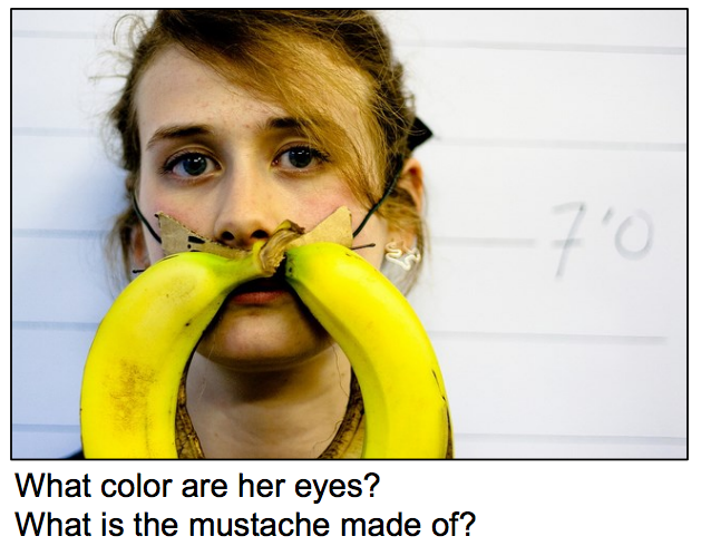
Figure 1. An example of free-form, open-ended question of the VQA task requiring common sense knowledge along with a visual understanding of the scene to answer questions.

There are many approaches to the VQA problem, one approach suggested jointly training the visual model and the language model, while the other recommended learning these two models separately and combining them at a later stage. In this project, we have decided to focus on various unexplored neural architectures that followed the second approach. The current state of the art model proposed by Lu, Jiasen, et al. in “Hierarchical question-image co-attention for visual question answering.” achieved 60.5% (with VGG) and 62.1% (with ResNet) on open-ended questions by using co-attention and question hierarchy. However, we did not consider these mechanisms in this project due to time constraints. Overall, the our main contributions of this project are: We explored different representations such as Convolutional Neural Network (CNN), Long-Short Term Memory network, Gated Recurrent Unit for the language models. We fine tuned several last layers of VGGNet-19 and ResNet and use them as the visual representation for the images. We also learned a front-end dilated CNN model. Finally, we tried different way of fusing information from the language model and the visual model, including simple concatenation, Multilayer Perceptron (MLP) and Bi-Linear outer product.

A short explanation of the main components in our networks:

Convolutional Neural Networks

Convolutional Neural Networks (CNNs) are a special kind of feed forward neural network where convolution layers replace the use of direct matrix multiplication operation by a convolution operation. Furthermore, the CNNs apply a pattern of local connectivity among the neurons belonging to adjacent layers. In addition, each filter of a layer is used across the entire image along with the weights and bias which drasticlaly reduces the number of parameters required as compared to the fully connected case. In our project, we used CNNs to extract features from thee images. As seen in recent literature, very deep networks provide rich representations of images with features extracted from different layers giving varied insights into the data. Thus, we decided to use the features generated by VGGnet and Residual Network (ResNet). The VGGNet is a deep feed forward CNN with 16 to 19 layers and same filter size of 3 for every convolution layer. While the ResNet shares VGGNet’s filter size, it can be trained with up to 34 layers due to the skip connections. These deep CNNs, however, are difficult to train from scratch and require large amounts of training data. Hence we used avaailable pre-trained networks and used these to fine tune the last few layers to provide us with our features. Recent work by insert proposed a new convolution module called dilated convolution that can aggregate multi-scale context without losing resolution by iteratively expanding the receptive fields. Their front-end model only required 8-dilated convolution layers, which are feasible to train and potentially has better representations of the images. Thus, we also considered this front-end architecture in comparison to the pre-trained VGGNet and ResNet features.

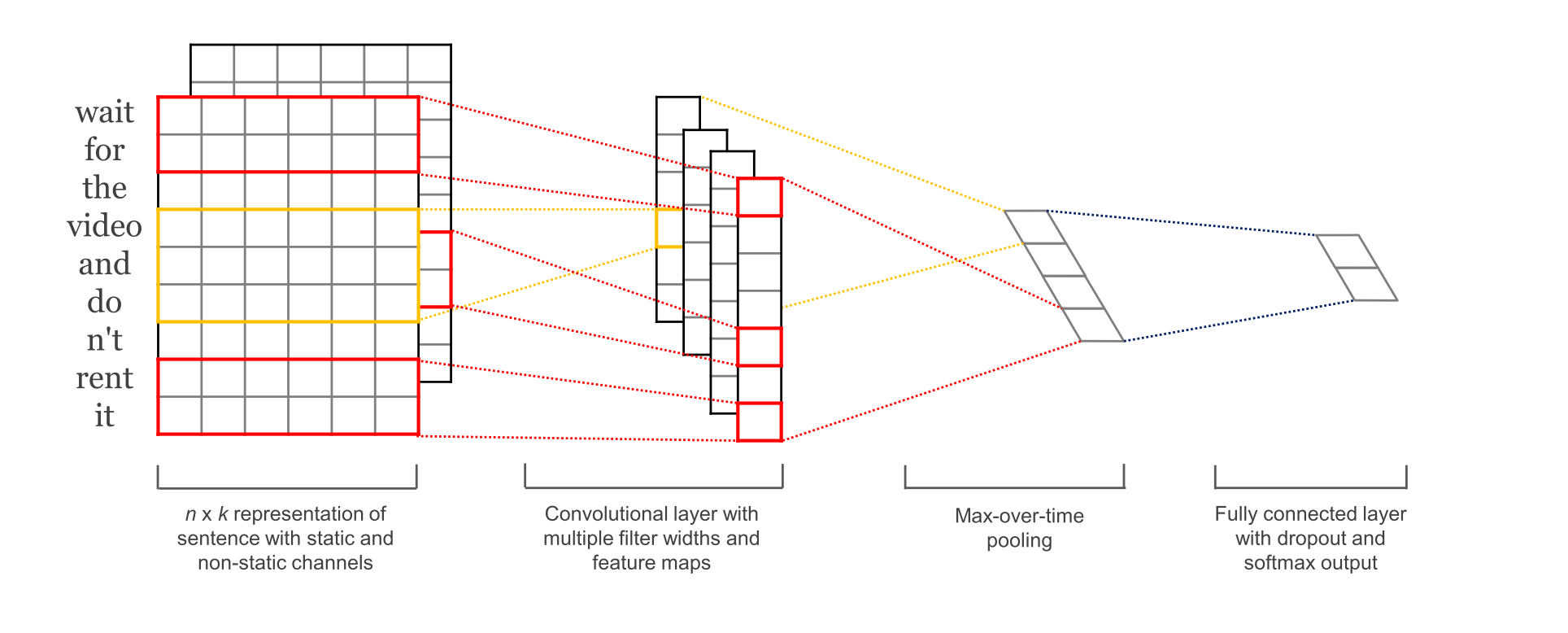
Figure 2. 1 Dimensional Convolution for text

More recently researchers have started to apply CNNs to text inputs as well. In insert, the author suggested the use of the 1-dimension convolution where the convolution mask is a vector instead of a matrix. Their work used a $s \times d$ representation of sentence of length $s$ and word features of $d$ dimension (Figure 2). The proposed convolution layer had multiple filter widths and feature maps and was followed by max pooling in time. The idea is to capture the most important feature, i.e. one with the highest value, for each feature map.

Long-Short Term Memory Network

Long-Short Term Memory Network (LSTM) is a variant of the Recurrent Neural Network (RNN). It was first proposed by Hochreiter and Schmidhuber in 1997 and has been successfully used for multiple applications in the language domain. Unlike the standard RNN, LSTM can not only collect recent information to perform predictions, but also can obtain information about “long-term” dependencies.

Unlike the standard RNN structure which only make prediction by computing a weighted sum of the input signal and applying a non-linear function such as tanh, the LSTM has a more involved structure. For each recurrent unit in LSTM, there are three gates: input gate, forget gate and output gate. For each time step t, the j-th LSTM cell will maintain a memory cell $c_{t}^{j}$, the output value $h_{t}^{j}$. The output value is computed as follows:

where $o_{t}^{j}$ is the output gate for this single cell at time $t$ at $j$th position, and it is computed using this equation where $\sigma$ is a logistic sigmoid function, and $W_{0}, U_{0}, V_{0}$ weight matrices.

The memory cell is also updated at each time step. It’s updated using the following equation, where

is the new memory cell, and $f_{t}^{j}, i_{t}^{j}$ are the corresponding forget and input gates.

As we can see from the above equations, each unit in LSTM decides whether to keep the previous information and to which extent to keep it, at each time step via the gates, i.e input gate, forget gate and output gate. So if LSTM detects some early important information, it will carry that information along with the whole prediction easily. So the long term dependency information can be captured.

Gated Recurrent Unit

Apart from LSTM, Gated Recurrent Unit (GRU) has been successfully used in language modelling due to its ability to capture long term dependencies while having fewer parameters. Both these methods combat the vanishing gradients problem that occur in deep networks. Several papers and blogs outline how they found GRUs faster to train, and easier to modify due to the less complex structure. Howevever there is no conclusive evidence as to which of the two is better in general so we decided to try both types.

Instead having forget and input gates, The GRU has a single “update gate” to replace them. And it also merges the cell state and the hidden state which result in a much simpler model than LSTM.

Same as LSTM, the output value from network is computed by the following:

As the above equation stated, the parameter $r_{t}^{j}$ is the reset gate and $\odot$ is element-wise multiplication. When $r_{t}^{j}$ is closer to 0, the reset gate effectively makes the unit act as if it is starting over, allowing it to forget all the previous information. And the parameter $z_{t}^{j}$ is the update gate, decides how much the unit updates its output. The candidate output value $\tilde{h_{t}^{j}}$ is computed as above too. Eventually, we get the representation for $h_{t}^{j}$.

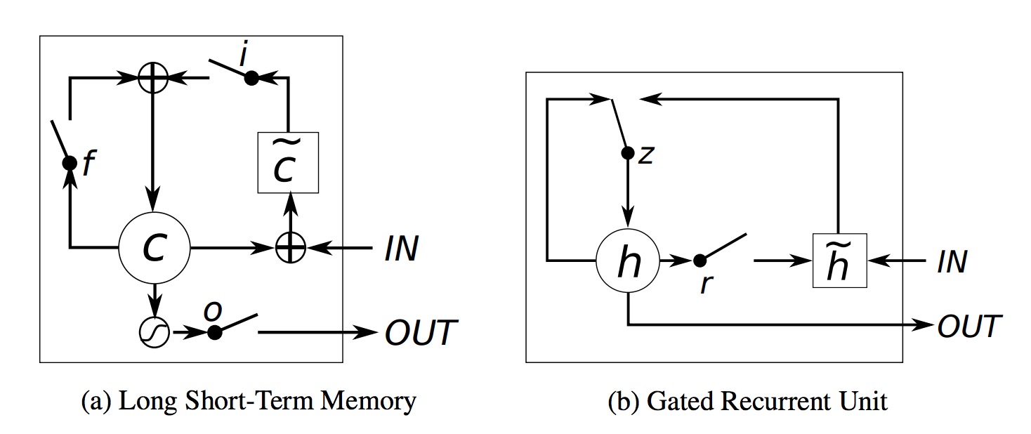
Figure 3. Graphical representation of LSTM and GRU

Our pipelines more specifically :

Visual representations

Ths part provides the features from the images. We experimented with four representations. V The activations from the last hidden layer of VGGNet were used as 4096-dimensional image representation.
R For ResNet, we took the pre-trained network, using representations from the last hidden layer then fine tuned it. Since the ResNet features were $4 \times$ larger than VGGNet, we added a Convolution layer with depth 512 and filter size of 3 to avoid memory overflows. We also added three fully-connected layers to form a final 4096-dimensional image representation. DV Inspired by the idea of the front-end model in Cite dilation paper , we used the features from VGGNet as input to a 8-layered dilated convolutional neural network. The last hidden layer representation were used as the 4116-dimension image representation. DR Same as DV, with VGGNet features replaced with ResNet features.

Language representations

This part provides a representation for the question. We experiment with several representations. For completeness, we also included the Bag-of-Words representation since the baseline model uses it. Bag-of-Words Question (BoW Q): This BoW representation took the top 1,000 words in the questions vocabulary to create a bag-of-words representation. It also create a 30-dim bag-of-words representation of the top 10 first, second, and third words in the questions as they contain important information such as question type. These representations are concatenated to create a final 1,030-dim embedding for the question. LSTM Q: An LSTM with one hidden layer is used to obtain 512-dim embedding for the question. The embedding obtained from the LSTM is the last hidden state representations of the LSTM. Each question word is encoded with 300-dim embedding from a pre-trained word2vec embedding which is then fed to the LSTM. Bi-LSTM Q: Similar to LSTM Q with a Bidirectional-LSTM in place of the LSTM. Because of its structure, the last state of the LSTM tends to agree more with the most recent input into it. In order to efficiently encoded the information from both past and future, we used the Bidirectional-LSTM. GRU Q: This model is simpler than LSTM model and has been found to surpass the LSTM in some cases, so we experimented with this structure too. CNN Q: Inspired by Kim Yoon’s work, using CNN for sentence classification \cite{kim2014convolutional}, we wished to try CNN with question as well. The input layer is composed with a sequence of size s of word embeddings of size \(d\). So the input feature map is a \(d * s\) feature map. Convolution layer is mainly designed for n-gram sliding. Three layers with various values of \(n\) were used for the convolution. Here, the filter is a \(d * n\) matrix, where n is the filter width and also the window size. After the convolution layers, there will be a standard max-pooling layer, which we used as the CNN representation for the questions.

Late fusion

We examine different ways to merge the image and question embeddings to obtain a single embedding. Fuse C: In this method we directly concatenate the two embeddings and then perform softmax classification. Fuse C + MLP: The image and the question embeddings are first transformed to match dimensions i.e., 512, 1024-dimensions by a fully-connected layer + tanh non-linearity. This is then concatenated and passed to a Multi-layer Perceptron (MLP) - a fully connected neural network classifier with 2 hidden layers of 1024-dim + tanh/relu non-linearity and a softmax layer to compute the distribution over K answers. Fuse B + MLP: The embeddings from two models are passed through several fully-connected layer + Relu non-linearity to learn bi-linear embeddings. Then, we take the outer product of the two embeddings and compute the final softmax classifier.

The entire model is then learned end-to-end with a cross-entropy loss. The pre-trained weights of the image channel are frozen except for the layers being fine tuned.

Experiments

Dataset

In this work, we evaluated our proposed models on the VQA dataset \cite{vqa}. In particular, the training set contained 215,375 question answer pairs and 82,460 images. While the testing set contained 121,512 question answer pairs and 40,504 images. The questions covered several sub-categories including yes/no, open-ended, number, and other. These questions require an understanding of vision, language and commonsense knowledge to answer. For each question, we had 10 corresponding free-form answer. We use the top 1000 most frequent answers as the possible outputs which spanned 86.54% of the training answers. We used the standard evaluation metrics and compare with the existing models. However, we did not use the VQA evaluating server and instead evaluated locally.

Setup

All of our models were implemented using Keras with a Tensorflow backend to fully utilize multiple GPUs. In all of our experiments, we used Adadelta \cite{adadelta} optimizer with careful chosen set of hyper-parameters for each proposed neural architecture.

Results

The overall results of the proposed models are shown in Table 1. We also compared our models with the baseline model in \cite{vqa} and the current state of the art work in \cite{hiecoatt}. All of our models were first sanity checked by over-fitting a small dataset and then trained on a small data set of roughly 10\% of the training data. We presented the details of tuning the hyper-parameters with relevant results for each model.

in progress..